When augmenting images during experiments, usually one wants to augment each
image in different ways. E.g. when rotating images, not every image is supposed
to be rotated by 10 degrees. Instead, only some are supposed to be rotated
by 10 degrees, while others should be rotated by 17 degrees or 5 degrees
or -12 degrees - and so on. This can be achieved using random functions,
but reimplementing these, making sure that they generate the expected values
and getting them to work with determinism is cumbersome. To avoid all of
this work, the library uses Stochastic Parameters. These are usually
abstract representations of probability distributions, e.g. the normal
distribution N(0, 1.0) or the uniform range [0.0, 10.0].
Basically all augmenters accept these stochastic parameters, making it easy
to control value ranges. They are all adapted to work with determinism
out of the box.
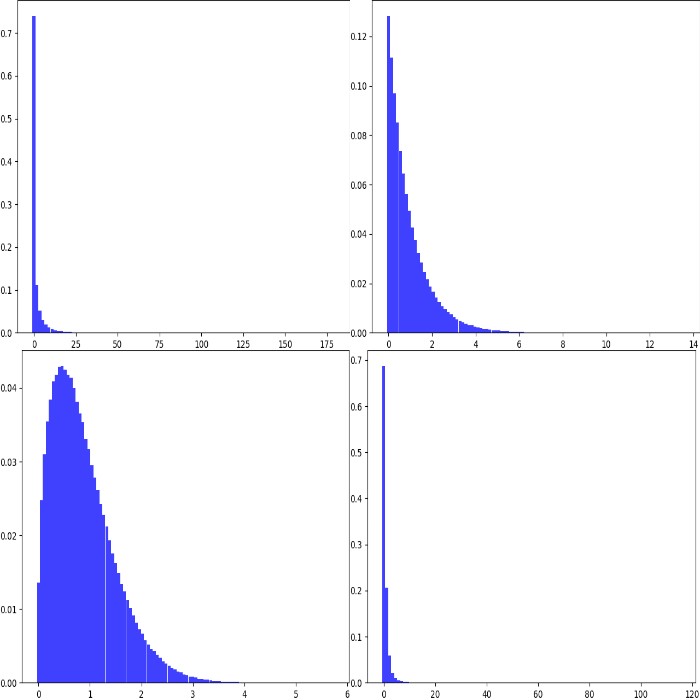
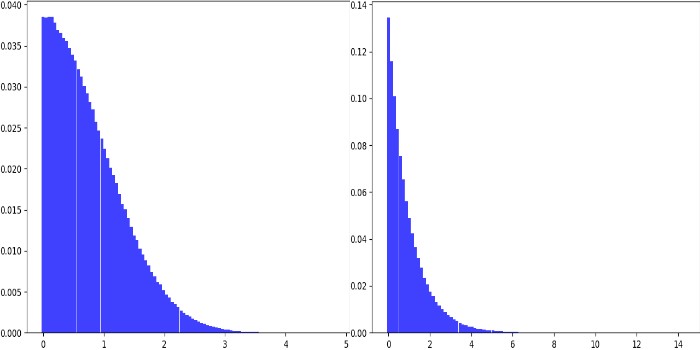
Blur each image by sigma, where sigma is sampled from the uniform range [0.0, 1.0). Example values: 0.053, 0.414, 0.389, 0.277, 0.981.
Increase the contrast either to 100% (50% chance of being chosen) or by 150% (30% chance of being chosen) or 300% (20% chance of being chosen).
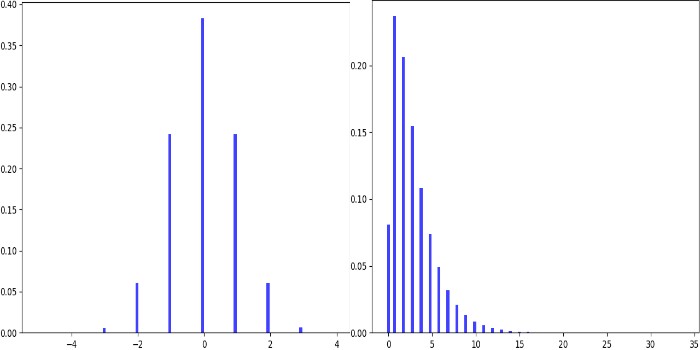
Rotate each image by a random amount of degrees, where the degree is sampled from the normal distribution N(0, 30). Most of the values will be in the range -60 to 60.
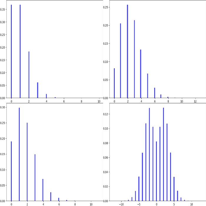
Translate each image by n pixels, where n is sampled from a poisson distribution with alpha=3 (pick should be around x=3).
As we cant translate by a fraction of a pixel, we pick a discrete distribution here, which poisson is.
However, we do not just want to translate towards the right/top (only positive values).
So we randomly flip the sign sometimes to get negative pixel amounts too.
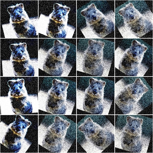
Add to each pixel a random value, sampled from the beta distribution Beta(0.5, 0.5).
This distribution has its peaks around 0.0 and 1.0.
We multiply this with 2 and subtract 1 to get it into the range [-1, 1].
Then we multiply by 64 to get the range [-64, 64].
As we beta distribution is continuous, we convert it to a discrete distribution.
The result is that a lot of pixel intensities are shifted by -64 or 64 (or a value very close to these two).
Some other pixel intensities are kept (mostly) at their old values.
We use Multiply to make each image brighter.
The brightness increase is sampled from a normal distribution, converted to have only positive values.
So most values are expected to be in the range 0.0 to 0.2.
We add 1.0 to set the brightness to 1.0 (100%) to 1.2 (120%).
The library supports arithmetic operations on stochastic parameters.
This allows to modify values sampled from distributions or combine several
distributions with each other.
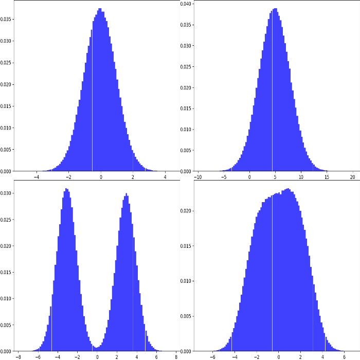
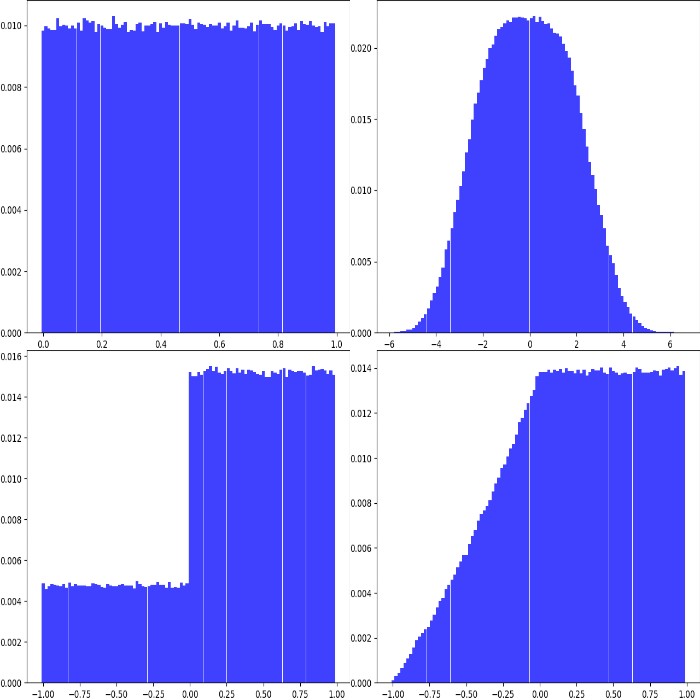
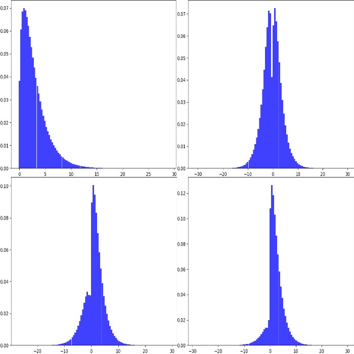
Add(param, val, elementwise): Add val to the values sampled from
param. The shortcut is +, e.g. Uniform(…) + 1.
val can be a stochastic parameter itself. Usually, only one
value is sampled from val per sampling run and added to all
samples generated by param. Alternatively, elementwise can be set
to True in order to generate as many samples from val as from param
and add them elementwise. Note that Add merely adds to the results
of param and does not combine probability density functions
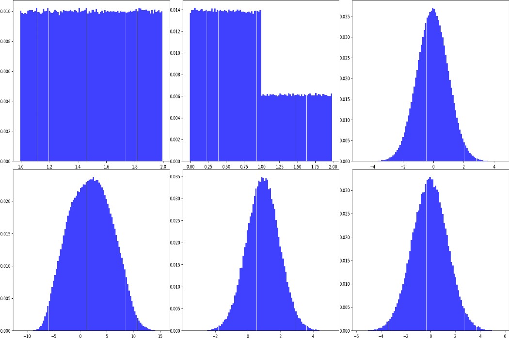
(see e.g. example image 3 and 4). Example:
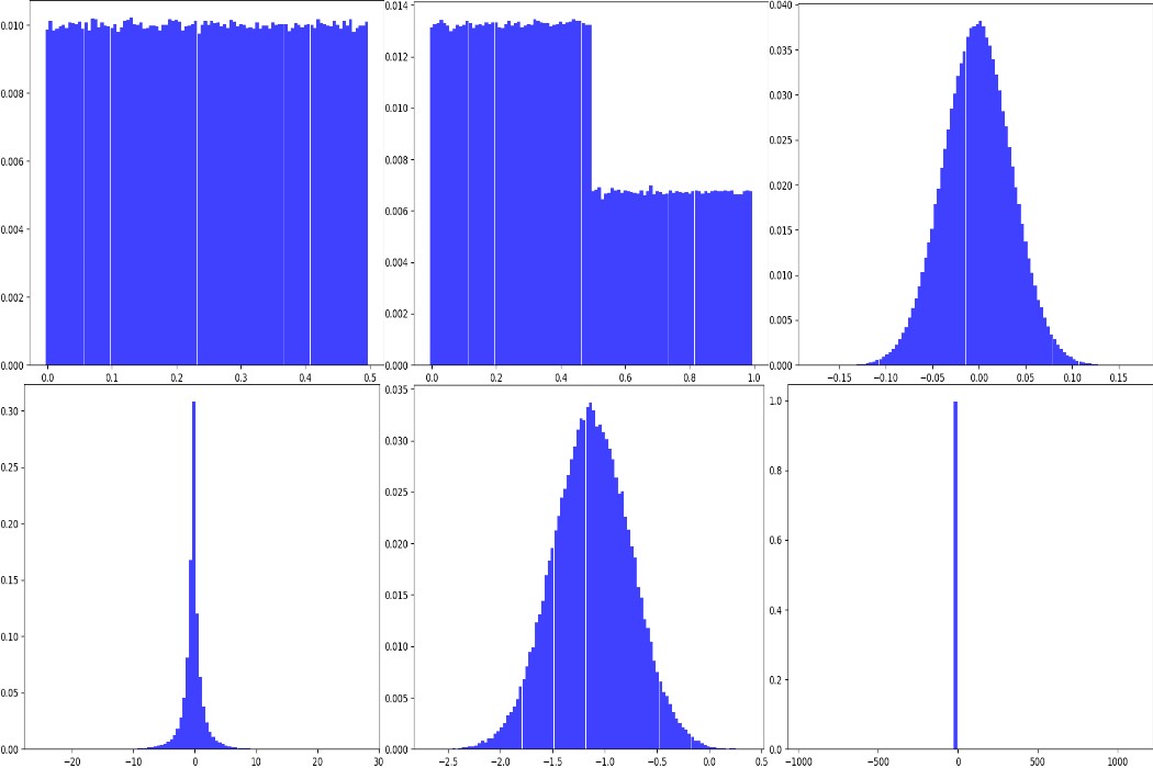
fromimgaugimportparametersasiapparams=[iap.Uniform(0,1)+1,# identical to: Add(Uniform(0, 1), 1)iap.Add(iap.Uniform(0,1),iap.Choice([0,1],p=[0.7,0.3])),iap.Normal(0,1)+iap.Uniform(-5.5,-5)+iap.Uniform(5,5.5),iap.Normal(0,1)+iap.Uniform(-7,5)+iap.Poisson(3),iap.Add(iap.Normal(-3,1),iap.Normal(3,1)),iap.Add(iap.Normal(-3,1),iap.Normal(3,1),elementwise=True)]iap.show_distributions_grid(params,rows=2,sample_sizes=[# (iterations, samples per iteration)(1000,1000),(1000,1000),(1000,1000),(1000,1000),(1,100000),(1,100000)])
Subtract(param, val, elementwise): Same as Add, but subtracts val
from the results of param. The shortcut is -,
e.g. Uniform(…) - 1.
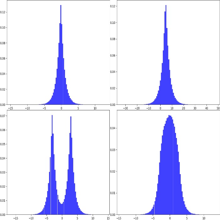
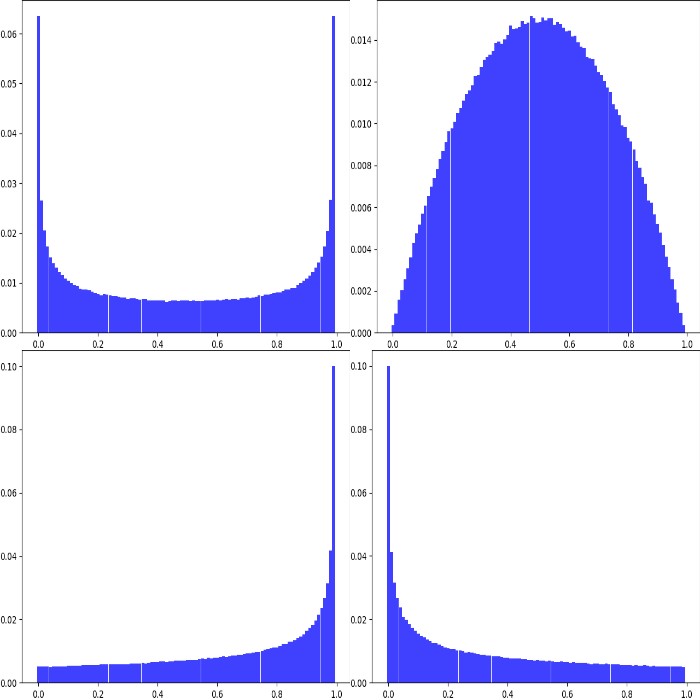
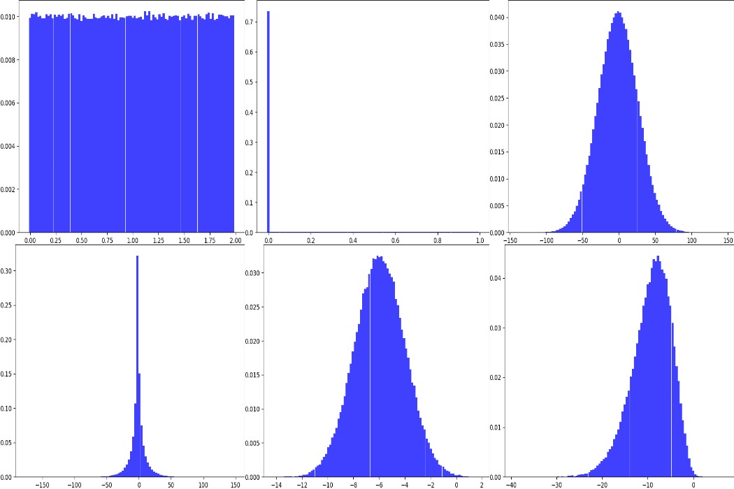
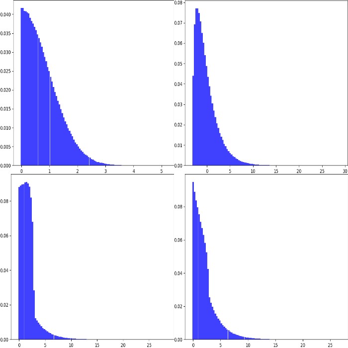
Multiply(param, val, elementwise): Same as Add, but multiplies val
with the results of param. The shortcut is *,
e.g. Uniform(…) * 2. Example:
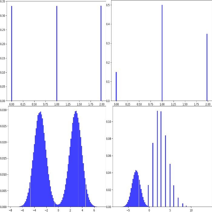
fromimgaugimportparametersasiapparams=[iap.Uniform(0,1)*2,# identical to: Multiply(Uniform(0, 1), 2)iap.Multiply(iap.Uniform(0,1),iap.Choice([0,1],p=[0.7,0.3])),(iap.Normal(0,1)*iap.Uniform(-5.5,-5))*iap.Uniform(5,5.5),(iap.Normal(0,1)*iap.Uniform(-7,5))*iap.Poisson(3),iap.Multiply(iap.Normal(-3,1),iap.Normal(3,1)),iap.Multiply(iap.Normal(-3,1),iap.Normal(3,1),elementwise=True)]iap.show_distributions_grid(params,rows=2,sample_sizes=[# (iterations, samples per iteration)(1000,1000),(1000,1000),(1000,1000),(1000,1000),(1,100000),(1,100000)])
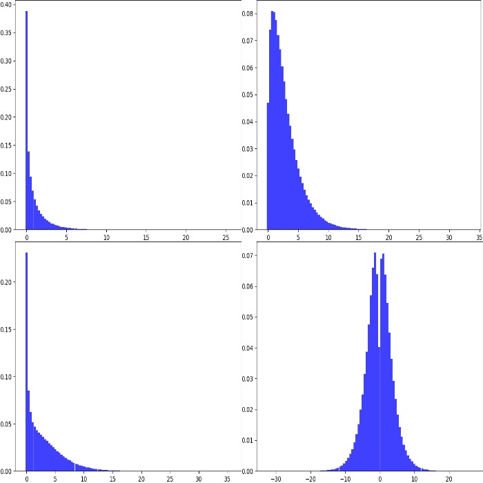
Divide(param, val, elementwise): Same as Multiply, but divides by
val. The shortcut is /, e.g. Uniform(…) / 2. Division by zero
is automatically prevented (zeros are replaced by ones). Example:
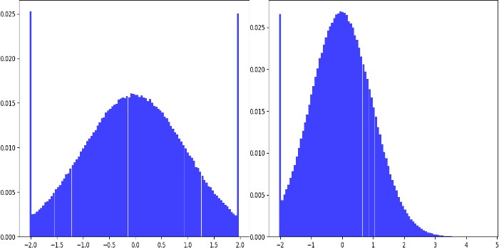
fromimgaugimportparametersasiapparams=[iap.Uniform(0,1)/2,# identical to: Divide(Uniform(0, 1), 2)iap.Divide(iap.Uniform(0,1),iap.Choice([0,2],p=[0.7,0.3])),(iap.Normal(0,1)/iap.Uniform(-5.5,-5))/iap.Uniform(5,5.5),(iap.Normal(0,1)*iap.Uniform(-7,5))/iap.Poisson(3),iap.Divide(iap.Normal(-3,1),iap.Normal(3,1)),iap.Divide(iap.Normal(-3,1),iap.Normal(3,1),elementwise=True)]iap.show_distributions_grid(params,rows=2,sample_sizes=[# (iterations, samples per iteration)(1000,1000),(1000,1000),(1000,1000),(1000,1000),(1,100000),(1,100000)])
Power(param, val, elementwise): Same as Add, but raises sampled
values to the exponent val. The shortcut is **. Example:
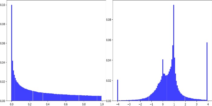
fromimgaugimportparametersasiapparams=[iap.Uniform(0,1)**2,# identical to: Power(Uniform(0, 1), 2)iap.Clip(iap.Uniform(-1,1)**iap.Normal(0,1),-4,4)]iap.show_distributions_grid(params,rows=1)
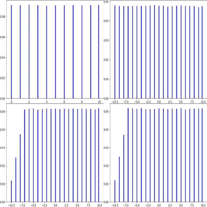
Deterministic(v): A constant. Upon sampling, this always returns v.
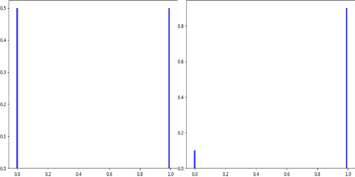
Choice(values, replace=True, p=None): Upon sampling, this parameter
picks randomly elements from a list values. If replace is set to
True (default), the picking happens with replacement. By default,
all elements have the same probability of being picked. This can be
modified using p. Note that values may also contain strings
and other stochastic parameters. In the latter case, each picked
parameter will be replaced by a sample from that parameter. This allows
merging of probability mass functions, but is a rather slow process.
All elements in values should have the same datatype (except for
stochastic parameters). Example:
Clip(param, minval=None, maxval=None): Clips the values sampled from
param to the range [minval, maxval]. minval and maxval may be
None. In that case, only minimum or maximum clipping is applied
(depending on what is None). Example:
RandomSign(param, p_positive=0.5): Randomly flips the signs
of values sampled from param. Optionally, the probability of flipping
a value’s sign towards positive can be set. Example:
ForceSign(param, positive, mode=”invert”, reroll_count_max=2):
Converts all values sampled from param to positive or negative ones.
Signs of positive/negative values may simply be flipped (mode=”invert”)
or resampled from param (mode=”reroll”). When rerolling, the number of
iterations is limited to reroll_count_max (afterwards mode=”invert” is
used). Example:
Positive(other_param, mode=”invert”, reroll_count_max=2):
Shortcut for ForceSign with positive=True. E.g.
Positive(Normal(0, 1)) restricts a normal distribution to only positive
values.
Negative(other_param, mode=”invert”, reroll_count_max=2):
Shortcut for ForceSign with positive=False. E.g.
Negative(Normal(0, 1)) restricts a normal distribution to only negative
values.
FromLowerResolution(other_param, size_percent=None, size_px=None, method=”nearest”, min_size=1):
Intended for 2d-sampling processes, e.g. for masks. Samples these in
a lower resolution space. E.g. instead of sampling a mask at 100x100,
this allows to sample it at 10x10 and then upsample to 100x100.
One advantage is, that this can be faster. Another possible use is, that
the upsampling may result in large, correlated blobs (linear interpolation)
or rectangles (nearest neighbour interpolation).